C++ - Beware What Lurks Beneath The Surface

C++ is a great programming language. It allows you to mix the most important programming paradigms like object orientation as well as generic, functional and structured programming. Another nice aspect is that the compilers are efficient and with some black template magick, you get some of these things for almost free at run time.

However, one of the greatest features of C++ can hurt you: When you write your own classes, they meld into your source code as if they were built-in types most of the time. However, always remember what is going on under the surface.

Today, I was hacking away at an OpenMP parallelization of a shortest-path algorithm (Highway Node Routing by Dominik Schultes) for my student research project. The algorithm needs to perform a lot of Dijkstra single-source shortest-path searches.

The existing code encapsulated the Dijkstra search in its own object class and the construction code had a single Dijkstra object to perform these searches:

class ConstructionClass {
public:
  ConstructionClass(Graph *g)
    : _graph(g), _dijkstra(g) {}
  
  void doConstruction() {
    // ...
    for (NodeID u = first; u != last; u++) {
      d.performSearchFrom(u);
      // ...
      d.clear();
    }
    // ...
  }

private:
  Dijkstra _dijkstra;
  Graph *_g;
};

This part of the parallelization comes almost for free: Use a Dijkstra object for each thread and you're done. OK, so I ended up with the following code in ConstructionClass::doConstruction() before adding #pragma omp parallel.

void doConstruction() {
  // ...
  for (NodeID u = first; u != last; u++) {
    Dijkstra d(_graph);
    d.performSearchFrom(u);
  }
  // ...
}

So far, so good. I compiled the program and let it run and the construction time went up from 2 seconds to more than 2 minutes! What was going on?

The problem was that the construction/destruction of the Dijkstra object for every loop took long: Whenever you do not use the new operator, you allocate objects on the stack and they get freed whenever the stack shrinks so it does not include the object any more.

Side node: Note that Java cannot do this — you cannot control where your object get created and because of garbage collection you cannot predict when the object is actually freed.

However, writing the code in C++ hid that fact from me since custom types look almost as built-in types. You could get the same problem with any class that does complex things in its constructor and destructor.

For example, the following two pieces of code are equivalent and memory allocation is expensive!

struct Table {
  Table(int size) {
    arr = new int[size];
  }
  
  ~Table() {
    delete [] arr;
  }
  
  int &operator[](const int index) {
    return arr[index];
  }

  int *arr;
}

// ...

for (int i = 0; i < MAX; i++) {
  Table t(MAX);
  // ...
}

and

for (int i = 0; i < MAX i++) {
  int *arr = new int[MAX];
  // ...
  delete [] arr;
}

Ruby's Multithreading: On Processes And Threads

Note that I made a grave error of thinking before writing this article: I forgot the copy-on-write page sharing of modern Unices. I added two paragraphs to this article that should clarify the point. Thanks for your comment, Alex.

Please note that I do not want to critizize Jason here. I am simply picking up this point from his presentation as a motivation of a topic that I wanted to write about since the issue with Ruby and threads occured. Also note that I actually like Ruby a lot and I am using it in almost all of my projects either for support scripts or as the main programming language: I am not anti-Ruby.

Today, the Riding Rails weblog linked to the slides of Jason Hoffman's tutorial Scaling a Rails Application from the Bottom Up in one of their entries.

While I do not want to doubt his expertise on scaling applications — he is the successful founder of Joyent, TextDrive and Strongspace — I stumbled over slide 115 of his tutorial which says

• I like that Ruby is process-based
• I actually don’t think it should ever be threaded
• I think it should focus on being as asynchronousand event-based on a per process basis
• I think it should be loosely coupled
• What does a “VM” do then: it manages LWPs
• This is erlang versus java

I have not attented his tutorial and thus I might misunderstand him. I might not be proficient enough in system and computer architecture. Nevertheless, I am wondering about the scalability of pure processes. There was a quite a discussion about Ruby and real kernel multithreading some time ago, but I did not read an article covering the same aspect that is discussed here: Memory Bus Saturation.

Thread, Process and Address Space

Let's recap the textbook definitions of threads, processes and adress spaces. Note that they do not necessarily map to what vendors call them or are consistent over all text books.

• A thread is pure activity, i.e. the information about the current position of execution (instruction pointer), the registers and the current stack.
• An address space is a range of addressable memory that is only accessible by activities that are allowed to read/write from it.
• A process consists of an address space and one or multiple threads.

OK, what does this mean? Each program that you run on your computer runs in its own address space if you are using a modern operating system, for example your web browser and your email client. Both applications (processes) appear to execute concurrently, i.e. you can download a web page and send an email at the same time. Even within each process, you can have multiple activities — threads. For example, your browser might download two images from a web site at the same time.

Your operating system executes the applications seemingly concurrently by using time slicing, i.e. assigning each process/task to the CPU for a short time and then assinging the next one.

Where is the real difference between processes and threads? Well, two threads within the same address space can access the same memory address at the same time. For example, both of the threads downloading an image can access the list of images for a website document.

The thread from your email applications cannot access this list. If the web browser and email client want to communicate, the operating system has to provide means for this. Communication could be done through files, pipes, sockets or message passing within the operating system.

User and Kernel Level Threads

Whee, that were a lot of new terms, eh? I have two other ones for you: kernel level threads and pure user level threads.

A kernel level thread (KLT) is a thread that the kernel is aware of, i.e. the kernel can decide which KLT will be schedule (assigned ot the CPU). Pure user level threads (PULTs) are not known to the kernel: One or more PULTs may run on top of a KLT and the kernel can only schedule the KLT. The decision which of the PULTs is scheduled is left to the user level scheduler in your application.

There are some tradeoffs between PULTs and KLTs and there are even hybrid models but the following problem remains: The kernel can only schedule KLTs to run on a given CPU. If you have more than one CPU/core then the kernel can schedule two KLTs to run concurrently. For example you could decompress two JPEGs at the same time in your web browser if you have two cores on your CPU.

Ruby only offers PULTs. What does this mean? This means that you cannot have one Ruby process with two threads running at the same time. You cannot, for example, let a Rails process generate two differently sizted thumbnails of an uploaded image at the same time. You cannot answer more than one request at the same time without stopping the other thread. You cannot do numerical computations on more than one core at the same time.

Ruby And 64 Core CPUs

So, we are coming closer to the problem that I see with Ruby and the upcoming 64+ core CPUs that DHH would welcome ``any day'' (so would most of us, right?). Try the following: Start the Ruby interpreter and a Rails console with ./script/console. The plain Ruby interpreter uses 1.2MiB and the Rails console session uses 28.42MiB on my Os X box; your mileage may vary.

I have not done any measurements but consider the following: Each of your Rails process needs 1.2MiB of memory for the interpreter and then more propably more than 20MiB of memory for your application instance. Some of this memory will be actively used in the inner loops of your program, let's make a conservative guess and say that each of your processes needs 0.5MiB of the address space most of the time. If you have a 64 core CPU then you need 32MiB of L2/L3 cache to access the memory quickly.

A typical L2 Cache on a Core 2 CPU with two cores is 4MiB of size. We could do some simple calculations and get that by the time, we have this 64 core processor, our L2 cache will have a size of 128MiB. After all, Wikipedia tells us that by 2007/2008 we will have 6MiB of L2 cache for two cores.

However: First, there are some physical limitations to the size of a cache hierarchy since electricity can only travel that fast. Second, as good engineers, we should consider whether we could cut down the memory requirements with sufficiently little work.

How would a multithreaded Ruby help to save memory? Well, the Rails console session used all of its memory by declaring classes and doing some initialization work. Most of this memory could be shared by multiple threads since you normally do not modify your classes on the fly in production systems. Your interpreter could be shared, too. By the estimates above, we could save more than 31MiB of cache for all the stack data we want.

Note that we could also save this memory with processes when forking at the correct time: When a process creates a child process, old Unices copied the whole address space. This is no longer the case: Modern Unices allow read access to the old address space from the new address space. When a memory location is written to by any process, the page will be copied into the new process' address space. Thus, if our Ruby/Rails classes do not change and we fork after Rails' initialization is complete, all of our 64 processes can share the same data.

I added this and the previous paragraph after the original article has been published because Alex reminded me of this fact in the comments. Thanks to him, the singlethreaded Ruby world is all fluffy again — mostly. A multi process system still has some traditional disadvantages like a higher cost of context switching (which could be negligible for interpreted languages like Python and Ruby). Additionally, we can ignore inter-process communication costs since Rails is share-nothing.

If we do not save this memory then we might hit the memory wall: The inner loops of the interpreter will fit into the program cache. However, the interpreter needs a lot of information for each executed line of Ruby code. Simply consider all the data that has to be accessed when a simple message has to be dispatched to an object...

What could happen is that we have to access a very large set of memory positions irregularly. If this happens on every core then we might get 64 cores accessing the bus at the same time because some piece of data is missing. This data might overwrite necessary information about a class in the cache and force this data to be reloaded again... If all cores shared the same data this would not be such big an issue.

Do you think my logic is wrong and my arguments are weak? Do you see a solution or workaround? I would be thrilled to read your comments.

Updates

• The original definition of a thread was missing that a thread has a stack. Thanks, DocInverter. (2007-09-26 17:39 MEST)
• Luckily, Alex was smart enough to see what I forgot: Modern Unices do copy-on-write sharing of address spaces when forking. I corrected the article. (2007-09-26 18:05 MEST)

Hitting The Memory Wall

Acknowledgement (2011-11-21): You should search Google for your blog titles before hitting "publish". When I wrote this article some years back, "hitting the memory wall" was just a term I had read some time earlier and internalized for myself as a standing term, like folklore. This was wrong. There is a paper from 1995 by WA Wulf and SA McKee with the same title: Hitting the memory wall that I was not aware of to this day. Thanks to sam in the comments for pointing this out. Sorry, for being late with the acknowledgement.

You have always ignored the internals of CPU properties like the number of registers, the exact format of CPU words, the precise format of intructions and of course the cache. I know you have (well, let's say I am sure about 99% of you out there). I ignored this for a pretty long time, too, when programming (although I was lucky enough to be forced to learn about the general principles at university).

And it has always been enough for you, right? Your enterprisy Java programs ran nicely, your beautiful literal Haskell programs zipped smoothly along and your Ruby and Python scripts ran with whatever speed the interpreter made possible. Your C(++) programs ran well, too, didn't they?

At least they did for me (ignoring bugs) - until now. I ignored the CPU internals, kept to common programmer's sense and best practice. I made sure my sorting algorithms ran in O(n · log(n)), searching ran in O(log n) and generally made sure that all algorithms algorithms were in polynomial time and the constants in big-O notation were small.

I thought I was happy and no problem would occur to me. And so you might think. Think again.

Ready, set, go...

I was working on parallelizing Counting Sort, a simple integer sorting algorithm that runs in linear time and needs O(n) additional space.

The algorithm is given an array of integers in the range of [0, max_key] and then works as follows:

• For each integer from 0 to max_key, count the number of occurences in the input array.
• Then, determine for each of these integers, where the first one will be written to in the sorted array.
• Third, copy the elements from the input array into a buffer array at the right positions.
• At last, copy the elements from the buffer back into input array.

Note that the algorithm is stable, i.e. the order within the elements with the same keys is preserved. This property is important for its application in the DC3 algorithm for linear time Suffix Array construction.

1  /* Use the Counting Sort algorithm to sort the range
2   *  [arr, arr + n). The entries must be in the range of
3   *  [0, max_key]. */
4  static void counting_sort(int* arr, int n, int max_key)
5  {
6    // counter array
7    int* c = new int[K + 1];
8    // reset counters
9    for (int i = 0; i <= K; i++)  c[i] = 0;
10    // count occurences
11    for (int i = 0; i <  n;  i++) c[arr[i]]++;
12 
13    // compute exclusive prefix sums
14    for (int i = 0, sum = 0;  i <= max_key;  i++)
15      {
16        int t = c[i];  c[i] = sum;  sum += t;
17      }
18 
19    // copy elements sorted into buffer
20    int *buffer = new int[end - begin];
21    for (int i = 0; i < n; i++)
22      buffer[c[arr[i]]++] = arr[i];
23 
24    // copy elements back into input
25    for (int i = 0; i < n; i++)
26      arr[i] = buffer[i];
27 
28    // copy elements back
29    delete [] buffer;
30    delete [] c;
31  }

Also note that we copy back the elements from the input instead of simply filling up the result array with the keys we determined earlier. The reason for this is that the input array could be an array of objects which are then sorted by a certain integer property/key.

...and crash!

So, where is the problem? Counting Sort! One of the simplest algorithms there is. Taught in undergraduate courses or in school! Can it get simpler than that? Where can the problem be?

I wanted to parallelize the DC3 algorithm using the shared memory with OpenMP. DC3 needs a linear time integer sorter to run in linear time and the reference implementation uses counting sort for it.

So I threw in some parallel instructions: Line 14-16 were executed for each thread, i.e. every thread got an equally (plus minus one) sized part of the input array and counted the occurences. Afterwards, the threads were terminated and the master thread calculated the "global prefix sums" so all threads got the right positions to write to. Then, lines 21-22 were parallelized again.

The parallelelized code can be found here.

OK, so far - since the sequential work is reduced to memory allocation and the global prefix sum calculation (aka rank calculation) involves very few additions there should not be a problem, right? (Let us ignore the copy-back step for this article.)

So I compiled the source on our Dual Xeon (each with 2 cores) machine with GCC 4.2 and level 3 optimization and ran some benchmarks. The maximum key was set to 127 (i.e. we could sort ASCII strings), the array size set to 16M (i.e. 64GB of data since ints are 4 bytes long on the architecture, filled with random integers) and the number of threads was varied from 1 to 4. The results are shown below (the line numbers correspond to the sequential code not the parallel one):

counting sort benchmark results, n = 2²⁸

no. of threads	1	2	3	4
line 14-17	30.20 ms	19.99 ms	29.74 ms	23.88 ms
lines 21-22	100.92 ms	59.61 ms	56.41 ms	55.78 ms

So, we get a speedup of about 1.5 with two threads but afterwards, there is no speedup at all. We should expect a speedup of n with n processors in these two parts since these sections were completely parallelized.

So, what the heck is happening there?

The von Neumann Bottleneck

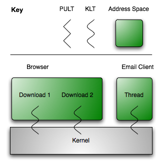
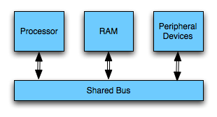
It's the von Neumann Bottleneck, baby! Today's SMP (Shared Memory Processing) systems are still built similar to the von Neumann machine. You were propably taught about it if you have a computer science background:

• The main memory is accessible via random access and stores machine words.
• The bus connects main memory, processor, peripherical devices. Only one connected entity can use the bus at any given time.
• The processor loads data and instructions from the main memory and executes it.
• There are peripherical devices for input and output (HDD, keyboard etc.)

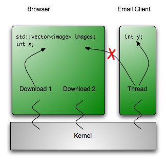
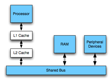
Today's computers do not work directly on the main memory, however, but normally on registers which can be accessed in one cycle. Read and write access to the main memory are cached in a cache hierarchy. The specs of the caches on the given machine were measured to be as follows:

memory hierarch specs for the Xeon 5140 system

-	L1 Cache	L2 Cache	Main Memory
size	32 KiB	4 MiB	8 GiB
latency [cycles]	3 cycles	9 cycles	133 cycles
latency [time]	1.28 ns	3.94 ns	56.95 ns

Additionally, the memory bus bandwidth in the system is 6.4 GB/s (however, as usual with bandwidth you will not be able to actually transfer more than half of that data per second in a real system).

So let us see if we can explain the behaviour with the knowledge about the architecture and these numbers in mind.

Lines 14-17 are executed 2²⁴ times in total and because ints are 4 bytes wide, this makes 2²⁶ bytes = 64 MiB transferred from memory if we only consider arr[] - c[] is small enough to fit into the processor's cache all the time (even one copy for each core).

With one thread (i.e. one processor working), 64 MiB get read in 30 ms which means that 2.133 GiB/s were read. With two threads working, the 64 MiB get read in roughly 20ms which manes that 3.2 GiB/s were read - the memory bus is saturated, our algorithm gets memory I/O bound and has to wait for the slow SD-RAM.

A Strange Phenomenon

Now, let us try to transfer that calculation to lines 21-22 - it should be pretty easy now. Again, we can assume that c[] can be kept in the level 1 cache all the time. This leaves reading arr[] and writing to buffer[]. Note that buffer[] is more or less accessed randomly (depending on the order of the values in arr[]). However, there are only 127 positions in buffer that are written to (limited by the size of c[]) and thus we can keep these positions of buffer[] in the L2 cache.

We would expect lines 21-22 to take twice the time than lines 14-17 because there are twice as much memory accesses. However, it takes thrice the time with two threads where we would expect the bus saturation. It gets even a bit faster with more threds although we would expect the bus to be saturated already! What is happening?

The image of modern computers we drew above was not really exact: Modern operating systems use virtual memory with paging to protect applications from each other and the kernel from user land:

Programs use virtual addresses to address their variables and these virtual addresses have to be translated into physical addresses. The data in the cache is addressed physically so access of main memory requires a resolution of a virtual address into a physical address. The addressing is done page wise, e.g. in chunks of 4 KiB. Each of these pages has a virtual base address which has to be mapped to its physical address (the place the page resides in RAM is called page frame).

The operating system has a table for each process that has the mapping from virtual page addresses to physical ones. This table resides in memory, too, and has to be accessed for each memory access. Parts of these tables are kept in a special cache: The so called Translation Lookaside Buffer (TLB). The TLB of the system is again separated into two levels, the faster one is approximately as fast as the registers, the slower one as fast as the L1 cache.

Let us explain our results with these numbers.

Since the page size of the system is 4KiB, we only have to look at the page table every 1024th memory access in lines 14-17. This very few times and we can neglect the access times since they are few and fast (since the L1 TLB is hit).

In lines 25-26, we transfer 128MiB in and out of the RAM. This should take us about 40ms but the lines take use 60ms. However, since access is almost random, we expect to look at the L2 TLB almost every time we want to access buffer[]. This means looking at it 2²⁴ times with 1.28ns each. This simplified calculation yields 21ms for the TLB accesses which seems right considered that we will hit the L1 TLB some times, too.

Whee, I do not know about you, but I would like to see a summary of all this to wrap my mind around it properly.

Summary

We examined the parallelization of counting sort, a simple linear time sorting algorithm. The algorithm could be parallelized well but the parallel parts did not yield the expected linear speedup. We considered current, modern computer architectures and could explained our experimental results with the specs of the machine we used and the knowledge of the architecture.

Note, ladies and gentlemen that we are crossing the border between algorithmics and system architecture here: Sometimes, actually implemented algorithms behave different from theoretical results (which indicated a lineare speedup).

So, what's next? We could try to kick our "slow" sorting algorithm into the virtual nirvana and replace it by another one. But which one should we choose? Counting sort needs exactly 4 · n + O(k) operations for an array with the length of n containing values from 0 to k. Any comparison based algorithm like Quicksort would need much more operations and parallelizing them comes at a pretty high overhead. Bucketsort exhibits the same non-locality when copying back elements and Radixsort needs another stable sorting algorithm like counting sort internally. If you, dear reader, know of a better linear sorting algorithm then please let me know since it would solve a problem for me.

We could use a NUMA machine where each processor has its own memory bus and memory. After splitting the input array, each processor could sort its part in its own memory. However, the final result composition would be slower since access to other processor's memory is slow and we have to go through one single bottlenecky bus again.

I hope you had as much fun reading this article as I had analyzing the algorithm and writing the article.

We are looking forward to your comments.

Updates

• I think that I have not made it clear enough above that the algorithm actually is cache efficient. Everwhere, memory is accessed, it is only accessed ones and in streams (every entry of c points to a part of buffer and this can be considered a stream). Each of these streams is read/written sequentially. This seems to have been hidden by the description of modern computers' architecture above.

Highly Efficient 4 Way Merging

Acknowledgements: This article is based on the work of Peter Sanders and Roman Dementiev. You can find the full source code presented here in their STXXL library (STL library for large data structures), Peter Sanders' paper and the accompanying source code. Warning: If you are of sensitive nature either regarding

• computer science theory
• highly practical program optimization

then I recommend you to stop reading this article at once. You might faint or something. Maybe, however, you can get a “bling” moment out of this article. Do you remember Mergesort from your introductory course in programming or computer science? An essential part of it is merging two already sorted lists into one as demonstrated in the animation below.

/* Merge two already sorted arrays where both are terminated
 * by 0x0fff ffff which may not appear *inside* arrays.
 */
void merge2(int a[], int b[], int result[]) {
  int i = 0, j = 0, k = 0;
  
  while (true) {
    if (a[i] <= b[j]) {
      result[k] = a[i];
      i += 1; k += 1;
    } else {
      result[k] = b[j];
      j += 1; k += 1;
    }
  
    if (result[k] == 0x0fffffff) return;
  }
}

If you are like me you do not think about Mergesort any more after understanding it and writing the exam it is relevant for. After all - people tell you that Quicksort has the same average run time and is normally faster and in place. This is not true in the general case but I'll keep that for another article. So, what is the deal about merging? If you complete your initial courses on algorithms and do not pursue algorithmics any further then chances are pretty good that you go ahead to things with more quickly visible and “tangible” results such as “enterprise” programs. But you shut your eyes to a pretty interesting part of computer science: Algorithmics. Merging gets interesting if you deal with I/O efficient algorithms: If you process data sets that do not fit your main memory any more then you will propably want to minimize I/O requests lest your shiny new Core 2 Duo processor will wait for your slow hard disk most of the time. Similar things have to be considered for the performance difference of your slow DRAM and the fast on CPU caches. Sequence Heaps are a highly I/O efficient (and cache efficient for data sets that fit into main memory) data structure for maintaining priority queues. Applications for priority queues include graph algorithms where you want to find the next largest node in your graph as fast as possible and graphs can get huge (think of all streets in Europe or North America, for example). The data structure described by Sanders requires an efficient R-way merger (where R is less than or equal to 4 for practicable sizes). Building a two way merger was pretty simple and we could extend this to a 4 way merger:

/* Merge four already sorted arrays where both are terminated
 * by 0x0fff ffff which may not appear *inside* arrays.
 */
void naive_merge4(int a[], int b[], int c[], int d[], int result[]) {
  int i = 0, j = 0, k = 0, l = 0, m = 0;
  
  while(true) {
    if (a[i] <= b[j] && a[i] <= c[k] && a[i] <= d[l]) {
      result[m] = a[i];
      m += 1; i += 1;
    } else if (b[j] <= a[i] && b[j] <= c[k] && b[j] <= d[l]) {
      result[m] = b[j];
      m += 1; j += 1;
    } else if (c[k] <= a[i] && c[k] <= b[j] && c[k] <= d[l]) {
      result[m] = c[k];
      m += 1; k += 1;
    } else { /* (d[l] <= a[i] && d[l] <= b[j] && d[l] <= c[k]) */
      result[m] = d[l];
      m += 1; l += 1;
    }
  
    if (result[m] == 0x0fffffff) return;
  }
}

OK, so we are all fluffy and set now, aren't we? If all arrays have the same length n then our naive_merge4 will run in O(n) and we cannot expect a better asymptotic runtime, right? We will not be able to improve on the asymptotic runtime since we have to look at least once at each element but each of our if statements has three comparisons! We have to do nine comparisons each time d contains the smallest element! Can we do better? We could use the comparison demonstrated in the following figure and reduce the comparisons to three in every case. 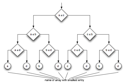Can we do even better? The answer is: Yes, we can - using Sander's code for four way merging:

template 
void merge4_iterator(
           InputIterator & from0,
           InputIterator & from1,
           InputIterator & from2,
           InputIterator & from3,
           OutputIterator to, int_type sz, Cmp_ cmp) 
{
  OutputIterator done    = to + sz;

#define StartMerge4(a, b, c, d)\
  if ( (!cmp(*from##a ,*from##b )) && (!cmp(*from##b ,*from##c )) \
      && (!cmp(*from##c ,*from##d )) )\
    goto s ## a ## b ## c ## d ;

  // b>a c>b d>c
  // a<b b<c c<d
  // a<=b b<=c c<=d
  // !(a>b) !(b>c) !(c>d)

  StartMerge4(0, 1, 2, 3);
  // [...] call StartMerge4 for every permutation of 0, 1, 2, 3

#define Merge4Case(a, b, c, d)\
  s ## a ## b ## c ## d:\
  if (to == done) goto finish;\
  *to = *from ## a ;\
  ++to;\
  ++from ## a ;\
  if (cmp(*from ## c , *from ## a))\
  {\
    if (cmp(*from ## b, *from ## a )) \
      goto s ## a ## b ## c ## d; \
    else \
      goto s ## b ## a ## c ## d; \
  }\
  else \
  {\
    if (cmp(*from ## d, *from ## a))\
      goto s ## b ## c ## a ## d; \
    else \
      goto s ## b ## c ## d ## a; \
  }

  Merge4Case(0, 1, 2, 3);
  // [...] call Merge4Case for every permutation of 0, 1, 2, 3

 finish:
   return;
}

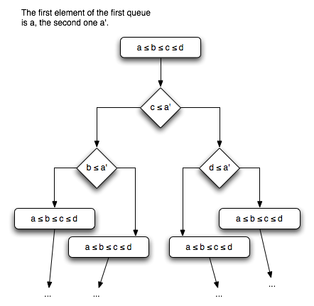
So, what's happening here? The macro Merge4Case generates the code for a specific ordering of the input streams from0, ..., from3. For each ordering, the next case can be found using only two comparisons (see the figure below). The macro StartMerge4 merely gets us started by jumping to the appropriate case. We have to do some work for initialization but after that we only have to do only two comparisons for each merge step! The instruction pointer (i.e. the current point of execution in the code) encodes the ordering of the input streams' ordering. Of course, there is a tradeoff: While naive_merge4 is only 20 lines long, the code merge4_iterator expands to much more than 200 lines. Of course, the native code does not correlate directly with the number of lines but the optimized variant will make the compiler create much more code than the naive merge method. The code for the optimized 4 way merger fits into the instruction cache and the tradeoff makes sense. However, we have to keep in mind that the code generated is dependent on the number of permutation of input streams. Thus, it is in O(R!). While 4! is only 24 a calculator or pen and paper give us 40'320 for 8!. I guess the code generated for an 8 way merger might not quite fit into the L1 instruction cache of the common CPUs out there (Wikipedia tells us that the Itanium 2 has a 16KB L1 instruction cache and a 256KB L2 cache that is used for both instructions and data). So, what can we learn from this?

• There are very elegant and powerful uses of the C preprocessor and the otherwise harmful GOTO.
• People at universities can write very pragmatic and efficient code.
• Algorithmics can be interesting (hopefully).

Updates

• Changed < to <= in the merge algorithms where it was wrong.

Simulation of Markov Decision Processes with enhanced generators in Python (with blood)

The language war will always go on and I consider myself as someone who has to promote the Python programming language no matter what happens (even though I know that there is no silver bullet.) Thus, I do have to use every opportunity to show the world how easy it is to connect formalisms of high scientific importance with not-so-important-but-still-cool language features.

Whatever.

Markov Decision Processes are big in machine learning. The whole field of reinforcement learning is based heavily on them since they are a good way to formalize environments in which an agent acts.

Python 2.5 brought a powerful new feature to the Python community: enhanced generators. If you want to give a function state you might consider overriding the __call__ method of your class - or you might want to go a way even more straightforward by using a generator function. If you are not familiar with Python's generators, you can read about them here.

Sending values into the generator is somehow more complex than it has to be if you do want to send in a value everytime you want to retrieve one. For example, you might want to have an adder that adds up numbers and always returns the current result:

def adder(n = 0):
  while True:
    inc = (yield None)
    n += inc
    (yield n)

That gives us in the REPL:

>>> a = adder()
>>> a.next()  # You have to forward the generator once
>>> a.send(2) # Sending in gives you a result
2
>>> a.next()  # Forward again
>>> a.send(3)
5

This can be eased with the following coroutine decorator:

def coroutine(func):
    def wrapper(*args, **kwargs):
        f = func(*args, **kwargs)
        f.next()    # Move on to the first
        def inner(message):
            while True:
                # StopIteration might be raised here, which is okay
                r = f.send(message)
                f.next()
                return r
        return inner
    return wrapper

Now you can use your adder much more easily:

>>> coAdder = coroutine(adder)
>>> a = coAdder(2)
>>> a(2)
4
>>> a(3)
7

We can use those features to simulate a Markov Decision Process. First let's recall a somewhat simpler definition: A Markov Decision Process (MDP) is defined by

• A set of states
• A set of actions
• Transition probabilities P(s, a, s') that describe the probablity of transfering from state s to state s' if action a is taken
• An initial state from the set of states

You can think of an MDP as a something that has a state and that you feed with actions - upon every action, the MDP transfers into a (possibly) new state. Let's have a look at an example:

Quentin is living together with his friends Bill and Beatrix. Bill and Beatrix have been going out together since some years, but today they have a serious argument . They run around the flat and scream at each other, swing their Hatori Hanzo blades and are about to cover the whole apartment in blood, gore and bones. Quentin is interested in not beeing in the same room with them since his two daikatanas are at the polisher. Bill and Beatrix keep chasing each other around the flat having a movie-like fight. The apartment is a little small and only has two rooms. Quentin has two actions: he can either switch the room or stay in the one he is at the moment.

There are two states - either Quentin is in the same room as the couple or he is in the other room. The fact that there are two different rooms does not matter for now, since we consider them only distinguishable on the fact who is in it.

Every time step the couple has a probability of 30% to switch the room. This leads to the following transition probabilities:

Same room, switch: 0.7 other room, 0.3 same room
Same room, stay: 0.3 other room, 0.7 same room
Other room, switch: 0.3 other room, 0.7 same room
Other room, stay: 0.7 other room, 0.3 same room

Of course, the best strategy for Quentin would be to switch rooms if they are in the same room and to stay if they are in the other room. The uber strategy "Leaving the flat" is not considered for educational reasons. ;)

How can this be implemented as a generator function? First we should think about how to represent the transition probabilites in Python, which can be done extremly easy with a dictionary:

 
transitions = {
  ('same room', 'switch'):  ((0.3, 'same room'), (0.7, 'other room')),
  ('same room', 'stay'):    ((0.7, 'same room'), (0.3, 'other room')),
  ('other room', 'switch'): ((0.3, 'same room'), (0.7, 'other room')),
  ('other room', 'stay'):   ((0.7, 'same room'), (0.3, 'other room'))}

This dictionary maps the (state, action) pairs to (propability, state') pair which is the probability that the next state is state'. The sets of states and actions are given implicitly by the probabilites.

To pick an item from a list depending on a probability, we can use this handy function:

from random import random
def randomPick(iterable):
   """Return one item of an iterable which consists of pairs (probability, item).

   The iterable is consumed."""
   # No check for correctness of probabilites to leave this to the programmer
   # and to not consume the iterable
   iterator = iter(iterable)
   s, i = 0.0, random()
   for prob, item in iterator:
       s += prob
       if i if i < s: return item

Now all we have to do to get our MDP is a very simple generator function:

@coroutine
def markovProcess(transDict, initialState):
    state = initialState
    while True:
        action = (yield None)
        state = randomPick(transDict[state, action])
        (yield state)

And this is as easy as it gets. This could of course be enhanced by using a function instead of a dictionary for the transition probabilites. But since the transitions are given by reference and not by value you can change the dictionary from the outside and the MDP will reflect this.

Ignoring folders with TODO Bundle in TextMate

TextMate's TODO bundle lets you keep track of the TODOs in your projects. You can mark a line to show up in the TODO list with FIXME, TODO or CHANGED. The following two images show a text file with these keywords and the resulting TODO list. The only problem is that if you keep a copy of Rails in vendor/, then the TODO plugin will also show the items in Rails (or any other external libraries and plugins you have in your project. This blog entry on exdolo.com describes how to get rid of the external items in your project with a sledgehammer: Add the vendor/rails folder to your global TextMate ignore list. However, there is a cleaner way: Open TextMate's Preferences Pane, go to Advanced » Shell Variables and the shell variable TM_TODO_IGNORE. You can set this variable to a regular expression as you would use it in Ruby (since the TODO bundle is written in Ruby). Et voilá: Rails-less TODO lists.

The Joys Of Floating Point Numbers

Sometimes, floating point numbers are the thing that futile hours of programming are made of. Whether they come as 32, 64 or any other precision you want, they can truly give you unnecessary and unexpected work if you do not use them correctly. The problem I stumbled over yesterday was the problem of rounding errors. Consider the following C snippet

double pi = 3.1415926535897932384626433832795;
double val = sqrt(pi) * sqrt(pi);

printf("pi  = %f\n", pi);
printf("val = %f\n", val);

which yields

pi  = 3.141593
val = 3.141593

Which is what we expected! val is the same as pi (the square is the inverse of the square root as we all know). However, the following C snippet shows the problem we run into:

if (val == pi) {
 printf ("pi == val\n");
} else {
 printf ("pi != val\n");
}

which yields

pi != val

So two apparently equal values are not equal any more! Where is the problem? It is in the precision of printf(), of course. We modify the first snippet so the printf() calls print the floating point values to more significant places

printf("pi  = %.16f\n", pi);
printf("val = %.16f\n", val);

and now we get

pi  = 3.1415926535897931
val = 3.1415926535897927

So how do we resolve this? Instead of comparing floating point values directly, we calculate their difference and make sure it is below a small value, for example 1e-9:

if (abs(val - pi) < 1e-9) {
 printf ("pi == val\n");
} else {
 printf ("pi != val\n");
}

which now gives us

pi == val

I guess most programmers are aware about the problems with floating point numbers and I have also known about the problem for a long time. What made me stumble, however, was that I trusted the printed value - which was inaccurate. As far as I know, there is no generic solution to the problem with floating point inaccuracies. You will get away with comparing whether the difference between two floating point values is smaller than a given value for comparing. In Ruby, you could hack the built in Float class with the following:

class Float
  def ==(value)
    self - value < 0.01
  end
end

This allows us to compare floating point values “fuzzily”:

>> Math.sqrt(2) ** 2 == 2.0
=> false
>> require 'floathack'
=> true
>> Math.sqrt(2) ** 2 == 2.0
=> true

However, I do not think that this is a good idea! Overwriting the == operator of the Float as above breaks its transitivity, i.e. we get the following (in-)equalities 1.99 == 2.00 == 2.01 but 1.99 != 2.01 Another idea would be only to compare the first n numbers after the point, e.g. consider 3.1415926535897931 to be 3.141 for n = 2. However, this does not help us if a floating point error gives us two values just next to a “boundary”, i.e. a result of 1.999 would not be considered correct if 2.001 was expected and we only cared about the result being “sufficiently close” to the expected value. So be careful when using floating point values are checking two of them for equality. Trouble will strike and most probably find some way to trick you into wasting time. An extensive, academic - and arguably dry - discussion of the implications of floating point arithmetics can be found in What Every Computer Scientist Should Know About Floating-Point Arithmetic, by David Goldberg.

SQLite gotcha

SQLite is great. No, really, I do mean it. If you ever need to work on structured data and editing it from the outside is a must, then SQLite is worth checking out and might be a superior choice to XML and will be a superior choice to your own proprietary format.

I cannot speak about performance - there are some outdated claims that SQLite is faster than postgres and mysql for the most common operations; but those benchmarks don't feature a single join, and that's where database implementation gets interesting and hard. I just cannot believe that SQLite stands up to any full scale DBMS.

I spent a few hours chasing down a bug in my own code after realising that I've been utterly stupid and put my parameters in the wrong order into my parameter list.

To boil it down, this is what happens in SQLite if I compare an integer field with a string in a WHERE part of a statement:

sqlite> CREATE TABLE my_favourite_numbers (number integer);
sqlite> SELECT * FROM my_favourite_numbers WHERE number = "foo";
sqlite>

You get no result. No error is thrown, like in Postgres:

# CREATE TABLE my_favourite_numbers (number integer);
# SELECT * FROM my_favourite_numbers WHERE number = 'bla';
ERROR: invalid input syntax for integer: "bla"

I know now what to look out for in the future.

First Post

Obviously, this is the first entry of the shining new Bitwiese Weblog. Feel warmly welcomed by these few bytes which propably travelled kilometre over kilometre from here to Blogger's servers and back again to you. This weblog is brought to you by Justin and me, Manuel. We hope to publish information related to the following

• programming
• computers in the widest sense
• computer science (prepare for some math, hehe).

So have fun and stay tuned.